
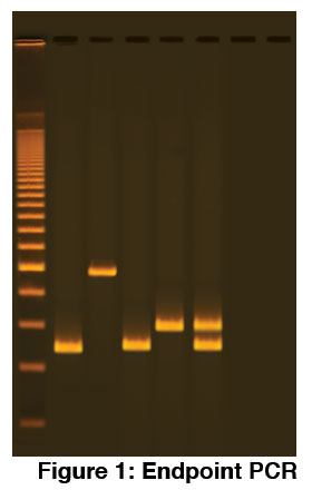
PCR exponentially amplifies copies of a DNA sequence. It’s great at producing more DNA for subsequent analysis. For example PCR combined with gel electrophoresis can tell us whether a particular loci is present or absent (Figure 1). It’s also somewhat of a black box – you put your sample in a thermal cycler, program in the cycles’ temperatures, and awhile later come and collect your product. We know what happens in between but we can’t see it happening in real time. Or rather we couldn’t until quantitative PCR, abbreviated as qPCR, came along. qPCR enables us to see the amount of amplified product as thafter every cycle.

What is qPCR?
A qPCR reaction is a PCR reaction with fluorescent dyes added (Figure 2). These fluorescent dyes let off a signal every time a strand of DNA is doubled. Consequently the amount of the fluorescence released during amplification is directly proportional to the amount of amplified DNA. This has some major advantages. By using a fluorescent reporter in the reaction, it is possible to tell if a sequence is present/absent without the second gel step. Also qPCR can accurately tell us the original amount of DNA in a sample. Such information is useful for monitoring the genetic expression of a particular gene and for detecting infectious diseases, cancer, and genetic abnormalities.
What does qPCR look like?
Theoretically all PCR reactions exponentially produce DNA. This means that there is positive linear relationship between the number of cycles and the log of the amount of DNA produced. In reality we can only see a small fragment of this line. In the beginning DNA amplification is too small to accurately observe. In the graph in figure 3 everything below the red line represents signals that are either undetectable or hard to measure because of background noise. At the end of a reaction reagents begin to run out which slows down the reaction. This is seen as a gradual flattening of the line. In between these two areas is the log linear phase. This is the region of the graph where the relationship between the fluorescence and the amount of starting material is the most consistent and measurable. Where the log linear line begins, e.g. where it intersects with the threshold line is known as the Cq (quantification cycle) point.

How does qPCR answer the “how much” question?
The Cq point is defined as the number of cycles required for the fluorescent signal to exceed background levels. It is inversely proportional to the amount of starting target nucleic acid in the sample – the more starting material the lower the Cq value for that sample. A Cq value for a sample can be compared to a standard curve to calculate the exact copy number of the original template. Creating this standard curve entails preparing a dilution series of known concentrations and then plotting the log of the initial template copy number against the Cq generated for each dilution. Comparing Cq values of unknown samples to this standard curve allows the quantification of the initial copy number.

Introduce your students to the power of qPCR with Kit #380 Discovering Quantitative PCR Amplification and Analysis or Kit #381 Break Through! Testing DNA Damage Using Quantitative PCR.
